Efficient Simulation Through Linear Algebra

I spent a lot of time working on a project in which physically plausible simulation of soft materials with pressure chambers was a key part,and in doing so, we managed to improve a part of our simulation by a significant amount. I was very happy with how this small part of the whole system turned out, and I've been wanting to share it for a while.

A fair warning though, we need to spend a little time setting up the context in order to see why this is a thing that can happen very naturally, as opposed to a magic algebraic trick that we can pull out of a hat.

If you haven't seen physically based simulations before, don't worry too much about the details. It helps if we can get on the same page regarding why we are even here in the first place, but the details of the context really doesn't matter for the point I'm trying to get across.

If you have seen physically based simulations before, also don't worry too much about the details. There isn't anything fancy going on here; no second order elements, no fancy time stepping, no dynamics, basically nothing that hasn't been around for 20 years¹. The trick is somewhat fancy though, to me anyways.

Finite-Elements

We wanted to simulate the behavior of a soft material with a certain geometry when we inject pressurized air into it. A simple way of doing so is by representing the geometry of the material with a tetrahedral mesh, and defining an energy that is a function of the deformation of those tetrahedra, or "tets". The nodal positions of the mesh are our "degrees of freedom": they are what we can move around, and the energy of the system is a function of those positions. You can imagine an energy function for each tet similar to²:

fn energy(nodes: [Node; 4]) -> f64 { ... }

If you are given any nodal positions, you can compute an energy from it. For instance, if a tet was supposed to have 1 volume, but it is stretched out to have 2 volume, it would make sense that it has a lot of energy, which it can "use"³ to return to it's preferred ("rest") position, of having 1 volume again. The energy function⁴ defines exactly how much the tet would want to return to some other configuration when deformed. By summing the energies for all the tets in the system, we get the total energy of the whole system.

You can also have other energies that adds into the whole system. Since we are dealing with a pneumatic system, we assign pressure forces to the faces of our mesh that are adjacent to the pressure chamber, such that the forces are proportional to the face area and the pressure. If we know how much gas is in the chamber (this is one our our degrees of freedom), and we know the volume of the chamber, we can compute the pressure using the ideal gas law⁵.

Finding Equilibrium

Having only this energy function, we can compute the forces that act on the nodes in our system as the direction in which they would have to move to decrease that energy. In other words, we let $$f = -\frac{\partial E}{\partial x}.$$ Note the minus sign: the gradient of a function is the direction in which it increases the most, and we would like it to decrease. This is also where notation gets a little messy: the $x$ above represents the positions of all the nodes, so it is really a vector in $\mathbb R^{3n}$ for a 3 dimensional system of $n$ nodes.

For a single tet, we have 12 numbers, namely the $x$, $y$, and $z$ coordinate of the four vertices. We can pretend that the energy function above reads

fn energy(nodes: [f64; 12]) -> f64 { ... }

With this, we see that $f_t$, the forces on a single tet, is also a vector of 12 numbers, which corresponds to the forces on the respective nodes in their respective coordinate, whichever way we flattened⁶ it in the first place⁷. $$f_t \in\mathbb R^{12}$$

We can use this information to move the nodes in our system in order to decrease the global energy of the whole system: loop over all tets, compute the forces from that tet to its four nodes, sum up the forces on all the nodes into one big vector $f\in \mathbb R^{3n}$, and move the vertices some amount $\eta > 0$ in this direction: $$x^{(i+1)} = x^{(i)} + \eta f.$$ This is called gradient descent, and it's not so great, at least not for these kinds of systems, because it takes a long time before it finds equilibrium. When $f=0$ we have reached equilibrium, and we're at rest.

Newton's Method

To improve convergence⁸ we can compute yet another derivative, namely $$ \frac{\partial^2 E}{\partial x \partial x} = \frac{\partial f}{\partial x},\qquad \frac{\partial f_t}{\partial x_t}\in\mathbb R^{12\times 12}$$ Now we've got $12 \times 12 = 144$ numbers, for each tet! Similarly to what we did above, we can combine all of these smaller matrices to one giant matrix⁹ that we'll call the Hessian $H\in\mathbb R^{3n \times 3n}$, and perform Newtons's method.

What we want to do with $H$ is find a direction $d$ such that $Hd = -f$ and then set our new node positions to be¹⁰ $$x^{(i+1)}=x^{(i)}+\eta d$$ Don't panic if this jumps out of nowhere, because it kind of does. Roughly speaking, what this means is that we pretend that our energy function is quadratic, because then this update will make us go straight to the minimum point, which in our case is force equilibrium. If the function is not quadratic (and it probably isn't), then we hope that we'll get closer, and indeed, as long as we start "sufficiently close" to the minima, we will.

Linear Systems

How do we "solve" $Hd = -f$ when we know $H$ and $f$? This is what we call a "linear system of equations", and is a workhorse of scientific computation, geometry processing, computer graphics, and many related fields. It is often written as the equation

$$Ax = b$$

or, if we choose dimensions of the variables (I chose 6 here) and write everything out explicitly:

$$ \begin{pmatrix} a_{1,1} & a_{1,2} & a_{1,3} & a_{1,4} & a_{1,5} & a_{1,6}\\ a_{2,1} & a_{2,2} & a_{2,3} & a_{2,4} & a_{2,5} & a_{2,6}\\ a_{3,1} & a_{3,2} & a_{3,3} & a_{3,4} & a_{3,5} & a_{3,6}\\ a_{4,1} & a_{4,2} & a_{4,3} & a_{4,4} & a_{4,5} & a_{4,6}\\ a_{5,1} & a_{5,2} & a_{5,3} & a_{5,4} & a_{5,5} & a_{5,6}\\ a_{6,1} & a_{6,2} & a_{6,3} & a_{6,4} & a_{6,5} & a_{6,6} \end{pmatrix} \begin{pmatrix} x_1\\ x_2\\ x_3\\ x_4\\ x_5\\ x_6 \end{pmatrix} =\begin{pmatrix} b_1\\ b_2\\ b_3\\ b_4\\ b_5\\ b_6\end{pmatrix} $$

The operation we want to do is find the $x$ given $A$ and $b$. That is, which $x$ (if any!) should I multiply $A$ with to get $b$? Algebraically, we can simply write $$x = A^{-1}b,$$ but this is very rarely done in practice because computing the inverse of a matrix is rather expensive¹¹. People have figured out that there are ways of finding $x$ without computing $A^{-1}$ explicitly, and it is this we mean by a linear solve.

For instance, in Julia we can use the \ operator for linear solves. Observe:

julia> A = rand(6,6) # Get a random 6x6 matrix (and hope it is full rank)
6×6 Matrix{Float64}:
 0.610793     0.0588659  0.90725   0.723158  0.480303   0.00631715
 0.10528      0.229984   0.536642  0.91345   0.650178   0.237762
 0.600606     0.24921    0.349393  0.626754  0.0971094  0.771216
 0.536192     0.0458314  0.541457  0.556307  0.132692   0.55307
 0.936709     0.215612   0.284619  0.304965  0.926599   0.719019
 0.000957923  0.852531   0.290136  0.151528  0.129307   0.0528658

julia> b = rand(6) # Get a random b
6-element Vector{Float64}:
 0.7716876359155332
 0.4285009788970344
 0.8110655185850537
 0.19638254649350662
 0.6621420580446692
 0.06633609289427767

julia> x = A \ b
6-element Vector{Float64}:
  2.77721146947569
  0.7894422416781481
 -2.7841498287174837
  2.5819747913641087
 -0.6223503841138821
 -2.1248845687489477

julia> A * x - b # If  Ax = b  then  Ax-b = 0
6-element Vector{Float64}:
 -1.1102230246251565e-16
  2.220446049250313e-16
  0.0
  5.551115123125783e-16
  1.1102230246251565e-16
  5.551115123125783e-17

There are many things to be said about solving linear systems, but there's only one more thing we'll need to know here: sparsity.

Solving Sparse Linear Systems

The picture below is the Hessian matrix $H$ of a one of these finite elements systems. The pixel at position i,j correspond to $H_{ij}$, and it is color coded so that blue means negative, red means positive, and gray is zero.

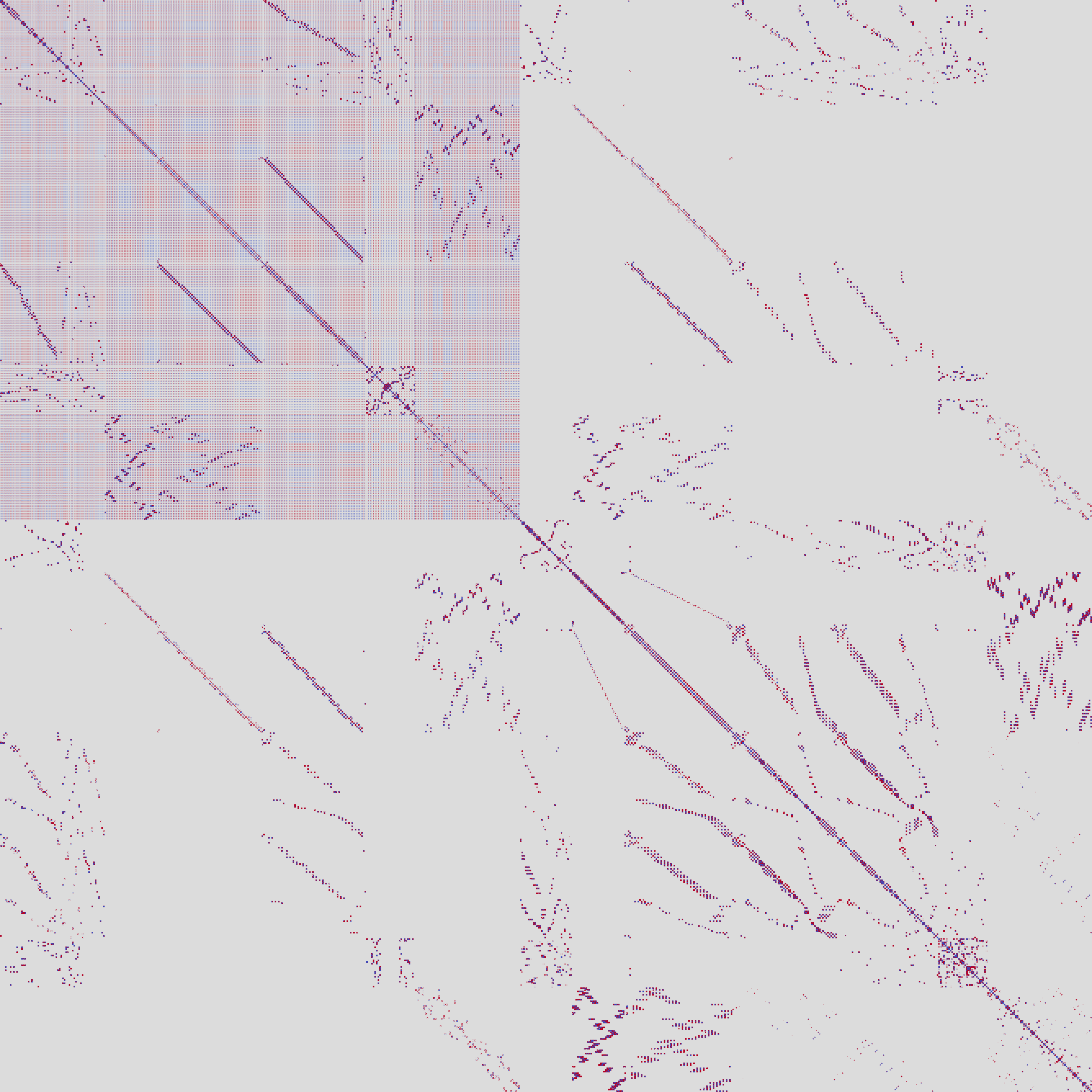
The noteworthy thing about this picture is the amount of gray: most pixels are gray. Since the Hessian quantifies how sensitive the forces on our nodes are to the position of the nodes themselves, this makes sense. Moving around a node on one side of the mesh does not change anything about the forces on the other side. That is, unless those nodes both are on the pressure boundary: in this case the volume is changed ever so slightly, which in turn changes the pressure, which in changes the forces on all of the nodes that are on the pressure boundary. These nodes correspond to the block we are seeing in the upper left corner or the picture¹².

Recall from above that there are a bunch of methods for solving these systems, but, perhaps obviously, any one of these methods will for sure need to look at each element in the matrix. If there are many elements in the matrix, there will be a lot of work; you can think of this as $O(n^2)$¹³ where $n$ is the number of degrees of freedom we have (the number of rows and columns in $H$). On the other hand, if most of the elements in $H$ are zero, we can store the matrix in a sparse format, so that any algorithm working on $H$ does not have to iterate over a whole lot of zeroes. It will still need to look at each non-zero number, but if we only have a constant number $c$ of entries in each row (or column), we only have a total of $O(cn)$ entries in total.

The problem, of course, is that the matrix in the picture above isn't really sparse, since it has this giant block of roughly $\frac{1}{4}n^2$ numbers in it.

... or is it?

Property vs. Representation

This brings us to the key of post. It certainly looks like the matrix is dense, and in general, there is no way of making a dense matrix sparse, since there is simply more information in a dense matrix. But maybe there is a lot of duplicate information in our matrix? To show what I mean, consider the matrix $$A = uv^\top\qquad\text{or equivalently }\qquad A_{i,j} = u_iv_j$$ or for some concrete numbers, consider this:

julia> u, v = rand(6), rand(6);

julia> u
6-element Vector{Float64}:
 0.17648645508411875
 0.9501460722894218
 0.7570256767954698
 0.9097476055645976
 0.7514042466862265
 0.2594892833200104

julia> v
6-element Vector{Float64}:
 0.9880351017724492
 0.7271356154478763
 0.29724548913210114
 0.7470357266014565
 0.8131233770317735
 0.26312703421677464

julia> u * v' # v' is Julia's way of transposing
6×6 Matrix{Float64}:
 0.174375  0.12833   0.0524598  0.131842  0.143505  0.0464384
 0.938778  0.690885  0.282427   0.709793  0.772586  0.250009
 0.747968  0.55046   0.225022   0.565525  0.615555  0.199194
 0.898863  0.66151   0.270418   0.679614  0.739737  0.239379
 0.742414  0.546373  0.223352   0.561326  0.610984  0.197715
 0.256385  0.188684  0.077132   0.193848  0.210997  0.0682786

The matrix is a "full" matrix of 36 numbers, but they all come from only 12 numbers¹⁴. In a sense, the matrix should be sparse, because it's only 12 numbers, but its representation is not sparse. If we can rewrite our $H$ above into a form that looks like this, maybe there's hope for speeding up the solves.

The way we compute pressure forces on the faces of the tets is first to compute the volume of the air chamber, compute the pressure using the ideal gas law, and apply the pressure on each face so that the force is proportional to both the pressure and the face area, and in the direction of the inward normal of the face. Roughly, following the notation I've used already, it looks like this¹⁵: $$f_p = p(x) n(x)$$ where both the pressure $p$ and the area scaled normal vector $n$ is a function of the node positions $x$. When we compute the Hessian entries $H_p$ for only the pressure forces, we use the product rule to get $$H_p=\frac{\partial f_p}{\partial x} = \frac{\partial p}{\partial x}(x)n(x) + p(x)\frac{\partial n}{\partial x}(x).$$ Writing it all out like this is useful since we can pinpoint exactly where in the formulas the density problem comes from. The term $\partial p /\partial x$ is dense, since it depends on the volume of the air chamber, and all nodes along the boundary of this chamber influences the volume if they move¹⁶ . But do note here that, similarly to the toy example above, we really only have $3n$ numbers in ${\partial p}/{\partial x}$, since for given $x$, $p(x)$ is only a single number --- the pressure --- so $\frac{\partial p}{\partial x} \in \mathbb R^{3n}$ (because $x$ is $3n$ numbers). Somehow this is expanded to $O(n^2)$ numbers in the process of assembly.

In fact, if we write $u=\partial p/\partial x$ and $v=n(x)$ then the first summand is just $uv^\top$. We use this to rewrite the computation of $H$ by first doing the pressure computation separately, and then the rest of $H$: $$H = H_p + H_r$$ ($r$ for rest) and then write the pressure terms as $$H_p = uv^\top + p(x)\frac{\partial n}{\partial x}(x)$$ and at last, we write the whole Hessian in a slightly more readable form as $$H = H_s + uv^\top,\qquad H_s = H_r + p(x)\frac{\partial n}{\partial x}(x)$$ This system is still as dense as before if we multiply out $uv^\top$ and add it all together, but we're not going to do that.

Solving The New System

Before we had the system $Hd = -f$ which we wanted to solve for $d$. Now our new system is the slightly less nice $$(H_s + uv^\top) d = -f$$ and it doesn't seem like we've made much progress.

What helps us is the Sherman-Morrison formula, which tells us how to invert a matrix of type $A + uv^\top$; see this and this post on solving these systems. The closed form solution includes inverting $A$ itself ($H_s$ in our case), but we can avoid computing this explicitly because we are not looking for the inverse of the matrix we have, we just want to solve the linear system.

For matrices that are easy to invert, the formula is useful for us; in particular, we choose $A=I$, and write out the inverse explicitly: $${\left(I + uv^T\right)}^{-1} = I - \frac{uv^T}{1 + u^Tv}.$$ Again, this does not help us directly yet, because in our case we have $H_s$ as the matrix inside the parenthesis, and not $I$. We will need to somehow massage it out.

The first step is to take our system $$(H_s + uv^\top)d = -f$$ and algebraically multiply in $H_s^{-1}$ from the left so that we get $$(I + H_s^{-1}uv^\top)d = -H_s^{-1}f.$$ Let's call $H_s^{-1}u=w$, or in other words, $H_sw = u$. Since $H_s$ is sparse we can easily solve for $w$, and insert this back into the equation: $$(I + wv^\top)d = -H_s^{-1}f.$$ Now we introduce a new variable, just to make this step easier: let $c = (I + wv^\top)d$. We haven't found $c$ yet, and we still don't know $d$, this too is just algebra. We are left with $$c = -H_s^{-1}f$$ or $$H_s c = -f$$ in which only $c$ is unknown. $H_s$ is still sparse, so we can solve for $c$. At last, we look at the definition of $c$ that we came up with. We have all quantities¹⁷ except for $d$: $$(I + wv^\top) d = c$$ and we already have a analytical inverse for this matrix, thanks to Sherman-Morrison. By inserting the inverse on the right and multiplying out (notice that we don't even have to construct the matrix that is the SM inverse!) we get: $$\begin{align} d &= {\left(I + wv^\top \right)}^{-1} c \\ &= (I - \frac{wv^\top }{1 + w^\top v}) c\\ &= c - \frac{w(v^\top c)}{1 + w^\top v} \end{align}$$ which is just two dot product, a scalar-vector multiply, and a vector-vector subtraction.

That's quite a mouthful, but in the end we have only solved two sparse linear system with the same matrix $H_s$, and done a few dot products at the end. We avoided the dense solve, and in fact, we avoided even constructing a new matrix.

The fact that we used the same matrix on both of the linear solves is also really important: linear solvers usually factorize the matrix in some way or another before they solve the system, for instance into an LU, LDLT, or QR factorization. When we have the factorization we can very easily solve the system, and so by solving multiple linear systems with the same matrix (and different $b$s) we only need to factorize once, so the second solve is really fast.

Quick Micro benchmark

What does this really give us? Instead of making a proper comparison from the simulation code base, I decided to hack together a small Julia program to illustrate. Here is the measured data of solving what basically amounts to the linear system above.

The data is generated from the following Julia code:

using LinearAlgebra
using SparseArrays

mod1p(n, m) =  ((n - 1) % m) + 1

# Compute a random sparse matrix in which each column has at most `k` entries
function randomsparse(n, k)
    A = zeros(n, n)
    for i=1:n
        ixs = rand(UInt32, k) .|> a->mod1p(a, n)
        nums = rand(k)
        A[ixs,i] = nums
    end
    sparse(A + I) # ensure we get a full rank
end
    
function doit(n)
    A = randomsparse(n, 5)
    u = rand(n)
    v = rand(n)
    b = rand(n)

    @time(begin # slow path
        slow = A + u * v'
        factor = factorize(slow)
        x = factor \ b
    end);

    @time(begin # fast path
        factor = factorize(A)
        w = factor \ u
        c = factor \ b
        x = c - w * dot(v, c) / (1 + dot(w, v))
    end);
end

The code for the fast path is a little more complicated than the straight-forward slow path, but overall, not by a lot. And the speedup we're getting is well worth it.

Conclusion

One of the reasons for why I really like this solution is that it's such a good example of good things happening because we looked closely at our problem. We already knew that linear solves would be the majority of the time spent in our pipeline. We also knew that sparse solves are quicker than dense solves. We also knew that our system felt dense due to the dependence of all the nodes along the air chamber boundary. Despite all of this, we managed to massage the problem we had from one dense solve into two sparse solves, and we got a significant speedup out of it.

This wouldn't have happened if we were content with the fact that "Linear solves takes up the majority of time in Newton's algorithm" (which is true; the linear solve is the bottleneck).

This wouldn't have happened it we looked at the Hessian and concluded that "The system is dense, therefore the solve will be slow" (which is true; dense systems are slower to solve).

Sometimes there are better solutions, but they require that we look closely at the problem at hand. Without looking closely in the first place, we wouldn't even have known that better solutions could exist.

Even though this example was full of math I really think the general sentiment translates well into programming, or completely different aspects of life. It is really hard to tell the difference between how something appears and how it really is¹⁸. I can't illustrate this with an example from your life, but I hope that having made the distinction here, you might come up with one.

Comments, questions, pointers, and prefactorized matrices, can be sent to my public inbox (plain text email only).

Thanks for reading.

This work is licensed under a Creative Commons Attribution-ShareAlike 4.0 International License