A Neat Approximation Algorithm

The algorithm and notation is based on section 9.3 of Williamson and Shmoys "The Design of Approximation Algorithms".

Let $G=(V,E)$ be a graph. A spanning tree $T$ of $G$ is a sub graph $T=(V, E')$ such that $T$ is connected and acyclic. Visually, you can think of it as a network that touches all vertices and doesn't contain and loops. Computing a spanning tree, even a minimal one if we have weights on the edges that we want to reduce, is easy¹.

Maybe we would like to ensure that no vertex is overloaded by having too many edges adjacent to it in $T$. We can look for spanning trees such that the maximum degree $\Delta(T)$ is bounded by some input number $k$. Is this problem difficult?

Yes, there is no polynomial algorithm that solves this in the general case². Consider what happens if we let $k=2$: now we are asking whether there is a Hamiltonian path in $G$, which is a well known NP-hard problem. To see why this is the same, note that if $\Delta = 2$ then the spanning tree can never branch out, since every vertex has at most one input and one output, and since it is connected we touch every vertex. Thus we get a simple path that touches every vertex exactly once --- a Hamiltonian path.

Okay, so we can't solve it exactly in polynomial time, but can we approximate it? It turns out yes, and with a surprising bound. Let $\text{OPT}$ denote the minimal maximum³ vertex degree in a spanning tree in a given graph. There is a polynomial algorithm that finds a spanning tree $T$ such that $\Delta(T)\leq\text{OPT}+1$. That is, it will either output a spanning tree that is optimal, or its maximum degree will be $1$ above the optimal.

We'll start off by stating a condition to have a tree with the bound above, then describe the algorithm, and then prove some claims.

Optimality Condition

First some notation. We are given a graph $G$ and consider a spanning tree $T$. Let $k=\Delta(T)$, $D_k$ be a non-empty set of vertices of degree $k$ in $T$, and $D_{k-1}$ be any set of vertices of degree $k-1$:

$$D_k \subseteq \{v\in V \mid d_T(v) = k \},\quad D_k\neq \emptyset$$ $$D_{k-1} \subseteq \{v\in V \mid d_T(v) = k-1 \}$$

$D_k$ are all of the bad vertices since they have the highest degree, and we want low degree vertices. $D_{k-1}$ are fine for now, but we need to be careful with them. We can't add any edges to these vertices, since then they'd be bad too.

Next, let $F$ be all edges in $T$ that touches either $D_k$ or $D_{k-1}$ (or both). These are the bad edges that we want to get rid of, because they are adjacent to the overloaded vertices in $D_k$ and $D_{k-1}$.

Last, let $C$ denote all connected components in $T$ if we were to remove all edges in $F$ from $T$. Note that we have exactly $|F|+1$ connected components: we start off by one component, since $T$ is connected, and for every edge we remove we split a component into two.

Here comes the condition:

If each edge in $G$ that connects distinct components in $C$ has at least one endpoint in $C_k\cup C_{k-1}$ then $\Delta(T)\leq\text{OPT}+1$.

A proof is at the bottom of the post (it is not very involved). This condition is almost all we need.

The High Level Picture

First a note on spanning trees. Since they span the entire graph and are acyclic, if we add a single edge to a spanning tree we will get a cycle⁴. Further, we can then remove any edge in the cycle and still have a spanning tree. At a high level, the operation we will do is exactly this: insert an edge adjacent to good vertices to make a cycle that involves some of the bad vertices, and then remove an edge that is adjacent to a bad vertex, making the total badness less.

Let's have some figures⁵ to make things a little more concrete.

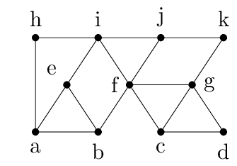
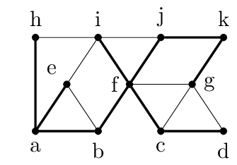
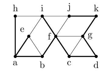
Say this is the graph $G$ with some spanning tree $T$ marked with bold edges. In the spanning tree, $a$ and $f$ are the bad vertices since $d_T(f)=4$ and $d_T(a)=3$. This means that we can choose⁶ $D_k=\{f\}$ and $D_{k-1}=\{a\}$. $F$ is all edges touching $a$ and $f$. Removing $F$ from the graph leaves us with the following graph, still with the edges from the spanning tree highlighted.

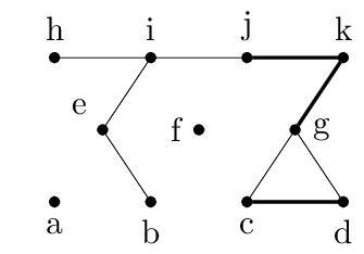
In this example, $C$ contains 8 components⁷: $C=\{ \{a\}, \{b\}, \{c, d\}, \{e\}, \{f\}, \{g, j, k\}, \{h\}, \{i\} \}$. Here the optimality condition above does not hold, since there are plenty of edges that connects components in $C$ that doesn't touch either $a$ or $f$; in fact, it just so happens that all the edges that are not spanning edges (i.e. bold) are connecting distinct components. This needs not be the case: imagine $(g,j)$ as an edge.

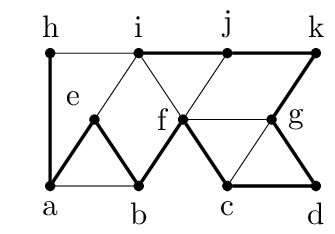
The idea of the algorithm is to see that the component $\{c,d\}$ and $\{g,j,k\}$ and be connected through the edge $(d,g)$⁸ (in blue below), and that this opens up the possibility of removing either $(b,f)$ or $(f,j)$ (in red below), which reduces the degree of $f$.

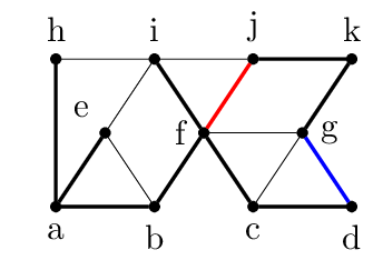
The resulting tree still spans the graph, and now we have reduced the maximum degree in the tree from $4$ to $3$. You can imagine doing the same trick with replacing $(a,b)$ in favor of $(b,e)$ and $(f,i)$ in favor of $(i,j)$. The resulting spanning tree would be optimal since its maximum degree is 2.

The Algorithm

The algorithm iterates until the optimality condition above is true. Let $k=\Delta(T)$ be the maximal degree of the spanning tree. In each step we aim to reduce one vertex of degree $k$ to $k-1$. If we reduce all such vertices we'll set $k=k-1$ and continue, aiming to lower the new $k$ even further. Initialize $D_k$ and $D_{k-1}$ to be all⁹ vertices of degree $k$ and $k-1$ respectively in $T$, and compute $F$ and $C$ as defined above. Find an edge that connects distinct components of $C$. If no such edge exist, we have our optimality condition. Let $e=(u,v)$ be this edge, and look at the cycle we get when adding $e$ to $T$.

Case 1

If the cycle does not contain a vertex $x\in D_k$, we don't do the swap. Instead we make a note that if we want to reduce any of the vertices in the cycle that is also in $D_{k-1}$ we can do so though $e$. Further, we'll remove all of these vertices from $D_{k-1}$, and update $F$ and $C$ accordingly. Effectively what this removal does is to merge all¹⁰ components that were connected to the cycle.

We have not done any real work yet, but we have made the set $D_k\cup D_{k-1}$ smaller, so maybe next time we'll get lucky. The downside is that we can no longer trust $D_{k-1}$ to contain all vertices of degree $k-1$. We removed the vertices from the sets, but we didn't remove any edges from the tree $T$. However, with the edge $e$ we have said that if we need to reduce the degree of one of these vertices, we can do so with $e$. Let's call this edge $e_u$ for a vertex $u$.

Case 2

If the cycle does contain a vertex $x\in D_k$, we want to add $e$ to $T$ and remove either of the two edges in the cycle that is adjacent to $x$. Now, if the degree of both $u$ and $v$ is less than $k-1$ all is well, since we've reduced the degree of $x$ from $k$ to $k-1$, and increased the degrees of $u$ and $v$ from something to something smaller than $k-1$ to something smaller than $k$.

However, if either of them is of degree $k-1$ we cannot do this. WLOG¹¹ let $u$ be the problem vertex. Now the setup in Case 1 pays off. Since $u\notin D_{k-1}$, but $d(u)=k-1$ we know that we have had Case 1 with $u$, and that $u$ was in $D_{k-1}$ along a cycle, and that we removed it. We also made the note saying that we can reduce the degree of $u$ upon request, though the edge $e_u$. Now we can add $e_u$ and remove either of the two edges adjacent to $u$ in the cycle that was formed by adding $e_u$. This makes $d(u)=k-2$ and we still have a spanning tree. Then we add $e$ and remove an edge adjacent to $x$, which increases $d(u)$ back up to $k-1$, and decreases $d(x)$ to $k-1$. If $d(v)=k-1$ as well we do the same with it.

We have successfully improved our spanning tree, since the number of vertices of degree $k$ has been reduced. Repeat this from the start by setting $D_k$ and $D_{k-1}$ to be all vertices of degree $k$ and $k-1$ and recomputing $F$ and $C$, until we hit the optimality condition.

There is one catch though. When we are reducing $u$ we are adding in the edge $e_u$ to the tree. How do we know that this edge will not make either of its endpoints' degree too high? The answer is that we don't! These vertices might also be of degree $k-1$, but then they, too, will have a designated edge $e_w$ that we can add to reduce $w$. We may end up with a chain of reductions, but this chain has to eventually terminate. See below.

And that's it! Some bookkeeping, component queries and merging, and basic graph operations, and we're left with a minimum degree spanning tree that is at most one from the optimal case, which is NP-hard.

Proofs

Here are proofs for the optimality condition and the termination and soundness of the cascading chain of reduction.

Proof of optimality condition

For brevity I will write "the set" for $D_k\cup D_{k-1}$.

We first find a lower bound for $\text{OPT}$. We have seen that $T\setminus F$ contains exactly $|F|+1$ components (this is the size of $C$). When the condition holds this is also true for $G$, since there are no edges connecting distinct components that doesn't also touch the set that are left in $G\setminus F$. This implies that any spanning tree in $G$ will need $|F|$ edges to connect them all. Furthermore, if we look at all the vertices in the set we know that their average degree must be at least¹² $|F| / |D_k\cup D_{k-1}|$, since $F$ is exactly all edges touching those vertices. The maximum has to be at least as large as the average, and so

$$\left\lceil\frac{|F|}{|D_k\cup D_{k-1}|}\right\rceil \leq \text{OPT}.$$

Now we find a bound on $|F|$. If we sum up the degrees of all the vertices in our set we get $k|D_k|+(k-1)|D_{k-1}|$, since the $D$ sets are exactly vertices of that degree. This sum can be more than the number of edges in $F$, since edges internal to the set will be counted twice. However, we also know that $T$ is acyclic, and so there can be at most $|D_k\cup D_{k-1}|-1$ such edges¹³, so we can add up the degrees of the vertices in the set and subtract the edges internal to the set to not double count. This gives us a bound on the number of edges touching the set¹⁴:

$$\begin{align} &k|D_k|+(k-1)|D_{k-1}| - \left(|D_k\cup D_{k-1}|-1\right) \\ =\ \ &k|D_k|+(k-1)|D_{k-1}| - |D_k| - |D_{k-1}|+1 \leq |F| \end{align}$$

Now we can combine the two inequalities by inserting the bound for $|F|$ into the bound for $\text{OPT}$:

$$\begin{align} \text{OPT} &\geq \left\lceil\frac{k|D_k|+(k-1)|D_{k-1}| - |D_k| - |D_{k-1}|+1} {|D_k| + |D_{k-1}|}\right\rceil \\ &= \left\lceil\frac{k(|D_k|+|D_{k-1}|) - \left(|D_k| + |D_{k-1}|\right) - |D_{k-1}|+1} {|D_k| + |D_{k-1}|}\right\rceil \\ &= \left\lceil k - 1 - \frac{|D_{k-1}|-1} {|D_k| + |D_{k-1}|}\right\rceil \\ &\geq k-1 \end{align}$$

Recall that $k=\Delta(T)$, so $\Delta(T) \leq \text{OPT}+1$.

Proof of termination of the algorithm

Since each step is either reducing $D_k$ or $D_{k-1}$ each iteration in the algorithm will eventually terminate, and since $k=2$ is the best possible maximal degree (unless we only have 1 or 2 vertices) we cannot reduce forever.

The less obvious part of the algorithm to terminate is the reduction of a $k-1$ degree vertex. Recall that in reducing a bad vertex $u$ with $d(u)=k$ we had to add an edge $(v,w)$ to the graph where $d(v)=k-1$, and this was done by adding in a second edge $e_v$. The problem is that $e_v$ might again be adjacent to a vertex of degree $k-1$, which will also have to be reduced. Now we show that this procedure will terminate. We do so by induction on the iteration number $i$, showing that when we mark a node as reducible (Case 1) we can perform the later reductions as well.

$i=1$: In the first iteration we have not marked any nodes as reducible through some edge, and so this terminates.

$i=l$: Let $u$ be the node we want to reduce, and $e=(v,w)$ the edge we reduce it with. WLOG let $v$ be the node we need to reduce, and $j$ the iteration in which we marked $v$ as reducible. By induction we can reduce $v$ from degree $k-1$ to $k-2$, and the same is true for $w$. How do we know that reducing $v$ using the edge $e_v$ doesn't mess up our reduction of $u$ with $e$? Because in marking $v$ as reducible we joined the two components that $e_v$ connected, and so in iteration $i$, the edge $v_e$ is internal to some component. In fact, the entire cycle formed by adding $v_e$ to $T$ is in that component. Since $C$ is not affected by the reduction of $v$, the reduction of $u$ via $e$ is still valid.

The only thing left to consider is that there is no chain of reductions that all add an edge to some vertex $x$, so that $k \leq d(x)$ after all reductions are done. This cannot happen: in fact, in a single iteration the set of edges that we add to the tree when reducing vertices are pairwise disjoint, and so any vertex will at most have its degree bumped once. Since the vertices of degree $k-1$ are already taken care of, no other vertex will suddenly have degree $k$, and so we are guaranteed progress.

To show disjointedness, let $u$ be reduced by the edge $e = (v, w)$, and assume that $v$ also needs to be reduced. Recall that, by definition, when we decided that $v$ is reducible through edge $e_v=(x,y)$, $e_v$ connected two different components. Further, we merged the components of the cycle that was formed by adding the edge $e_v$ into a bigger component $C_v$, which contains both the two components that $e_v$ connected and $v$ itself. This is one of the components that $e$ connects, and it does so through $v$, so we know that $e$ and $e_v$ are disjoint. Now, if either $x$ or $y$ also needs to be reduced, say $x$, that will be through $e_x$, which will, by the same logic, be internal to the component $C_x$, which does not contain neither $u$, $v$, or $w$, so $e_x$ is also disjoint from both $e$ and $e_v$¹⁵.

Conclusion

We've seen an algorithm that finds a spanning tree that minimizes the maximum degree of the tree up to an error of 1. The original paper where this was taken from, link here, is called "Approximating the minimum degree spanning tree to within one from the optimal degree" by Fürer and Raghavachari. I didn't actually read the paper, just the book chapter mentioned in the beginning.

I thought the algorithm was especially neat due to the bound, since approximation algorithms often are multiplicative factors off the optimal solution, for instance with a factor of 2 or 1.5. It is interesting that finding a spanning tree with maximal degree 2 is NP-hard, but that there is a polynomial algorithm that will find a spanning tree of maximal degree of 2 or 3 if the graph is Hamiltonian.

I haven't tried to implement this, but from what I can tell it should not be too difficult. It would be interesting to see some statistics on the performance of this algorithm on a corpus of graphs that are known to be Hamiltonian. Things like:

• How long do the reduction chains become?
• How many iterations are required before we reach optimality?
• How often do we get the optimal tree?
• How does $|F|$ change during the lifetime of the algorithm?
• How does $C$ change during the lifetime of the algorithm?

and probably many other thing. If you know of any work on this or have any ideas yourself, feel free to send it to my public inbox (plain text emails only).

Thanks for reading.

This work is licensed under a Creative Commons Attribution-ShareAlike 4.0 International License